
Introduction to Image Processing
A short introduction to Digital Image Processing for Computer Vision

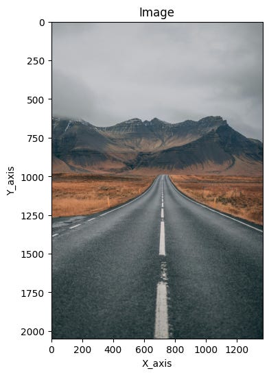
In the realm of computer vision, the concept of an image takes on a precise and technical meaning. Unlike the broad artistic or photographic interpretations, computer vision focuses on digital images—structured data representations that encode spatial and color information. These images are not continuous like those we perceive with our eyes, but rather discrete, meaning they consist of individual units or pixels arranged in a grid.
A digital image can be thought of as a matrix of values, where each element corresponds to a specific location and intensity. This spatial layout is typically defined within a two-dimensional Cartesian coordinate system, and the intensity values represent color or brightness at each point. The image, denoted as ( I(m, n) ), reflects the response of a sensor—such as a camera—at fixed positions across the grid.
This discrete image is derived from a continuous spatial signal ( I(x, y) ), which represents the real-world scene in its natural, uninterrupted form. The transformation from continuous to discrete is known as discretization, a fundamental process in digital imaging. Through discretization, the continuous signal is sampled at regular intervals, allowing computers to store, process, and analyze visual data efficiently. This foundational concept enables a wide range of applications, from facial recognition to autonomous navigation.
Digital image processing is the most widely recognized form of image manipulation in computing. It involves the use of algorithms to perform operations on digital images, often with the goal of enhancing them or extracting useful information. This discipline plays a foundational role in the broader field of computer vision, where machines are trained to interpret and understand visual data.
Both image processing and computer vision begin with the same starting point: an input image. However, their objectives diverge significantly. Image processing focuses on transforming the image itself—adjusting contrast, removing noise, sharpening details, or converting formats. The result is typically another image, often improved or altered for a specific purpose.
In contrast, computer vision aims to derive meaningful insights from the image. Its output is not another image, but rather data—such as object locations, classifications, or measurements. For example, a computer vision system might identify faces in a photo, detect motion in a video, or recognize handwritten text. While image processing can be a preliminary step in computer vision workflows, the two fields serve distinct roles in the digital analysis of visual content.
Why is image processing difficult?
Image processing presents a range of challenges that stem from both the nature of visual data and the complexity of interpreting it. One of the most fundamental difficulties arises from the dimensional reduction that occurs during image capture. Devices like cameras—and even the human eye—project a three-dimensional world onto a two-dimensional plane. This transformation results in a significant loss of spatial information, making it harder to infer depth, shape, and context from flat images.
Another major hurdle is the interpretation of images. Humans perform this task effortlessly, drawing on years of accumulated knowledge and experience to make sense of visual scenes. Our brains can recognize patterns, infer relationships, and apply reasoning to new situations based on familiar cues. In contrast, computer vision systems must be explicitly trained to replicate this process, often relying on vast datasets and sophisticated algorithms to approximate human-level understanding.
Noise is yet another complicating factor. Every real-world measurement—whether from a camera sensor or another imaging device—contains some degree of uncertainty. This noise can distort the image and obscure important details, requiring robust mathematical techniques to filter and correct the data without losing valuable information.
Finally, the sheer volume of data involved in image and video processing adds to the complexity. High-resolution images and continuous video streams demand substantial computational resources. While modern hardware has made these tasks more accessible, especially with consumer-grade devices, managing and processing such large datasets efficiently remains a core challenge in the field.
Image processing levels
Image processing is often structured into a hierarchy that distinguishes between low-level and high-level techniques. This classification helps clarify the nature of the operations being performed and the complexity of the algorithms involved.
Low-level image processing focuses on direct manipulation of the raw image data. These methods include tasks such as image compression, noise filtering, and sharpening. The goal is to enhance or prepare the image for further analysis, and the data used at this stage closely resembles the original input. These techniques are foundational, often serving as the first step in more complex visual workflows.
High-level image processing, on the other hand, operates on a more abstract plane. It is driven by knowledge, goals, and strategic plans, often leveraging artificial intelligence to simulate human cognition. This level of processing aims to interpret the image, extract meaningful features, and make decisions based on the visual information. High-level computer vision systems strive to replicate the human ability to reason and understand, transforming raw pixels into actionable insights.
Understanding Image Representation in Computer Vision
Recognizing and interpreting images is a remarkably complex task for computers. Unlike humans, who effortlessly draw on years of visual experience and contextual understanding, machines must rely on mathematical representations and algorithms to make sense of visual data. This challenge begins with how images are represented digitally.
At the core of every digital image is the pixel—the smallest unit of visual information. A pixel encodes data about color and intensity at a specific location in a two-dimensional grid. In mathematical terms, a pixel is often represented as f(hr,vr), where hr denotes the row and vr the column in the image matrix. This notation captures the amplitude or value of the pixel at that particular coordinate.
However, the pixel value itself is influenced by two key physical properties: illumination and reflectance. Illumination, denoted as a(hr,vr), refers to the amount of light falling on a surface, while reflectance, b(hr,vr), describes how much of that light is reflected back. Together, these factors determine the final appearance of each pixel, making image interpretation a nuanced process that requires careful modeling of real-world lighting and material behavior.
This layered complexity is one reason why image representation—and by extension, image recognition—is such a demanding task in computer vision. It requires not only precise data handling but also sophisticated algorithms capable of bridging the gap between raw pixel values and meaningful visual understanding.
RGB Image Representation and Its Challenges
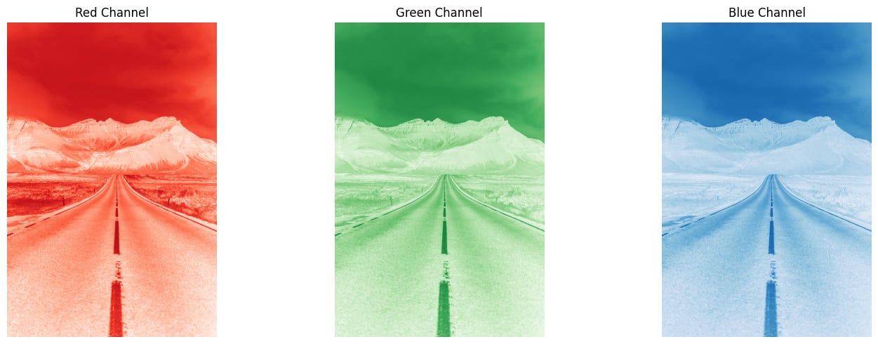
Color images in digital processing are typically represented using the RGB model, where each pixel is defined by a triplet vector corresponding to red, green, and blue components. These three values form a linear combination of basis colors, allowing the full visible spectrum to be encoded. Conceptually, an RGB image can be viewed as three separate 2D planes—one for each color channel—resulting in a 3D array of dimensions ( C \times R \times 3 ), where ( C ) is the number of columns and ( R ) the number of rows.
Each pixel in a true-color image holds three numerical values, one for each channel. These channels can be easily separated and visualized individually, but it’s important to understand that most real-world colors are blends of all three components. For instance, an object perceived as blue will appear brightest in the blue channel, yet it will also contain lesser contributions from red and green. This blending is a fundamental aspect of how colors are formed and perceived.
A common misconception is that color-specific objects only appear in their respective channels—blue in blue, red in red, and so on. In reality, color perception is more nuanced. Even strongly colored objects have traces of other channels, which contribute to shading, texture, and realism.
In digital image processing, the RGB model is based on the CIE color standard of 1931 and is optimized for graphical displays. However, one of its limitations is perceptual nonlinearity. This means that changes in RGB values do not always correspond to consistent changes in perceived color. For example, increasing the red component may not produce a visually proportional shift in hue or brightness. This nonlinearity poses challenges for tasks like color correction, segmentation, and enhancement, where human perception must be closely matched by algorithmic adjustments.
HSV: A Perceptual Approach to Color Representation
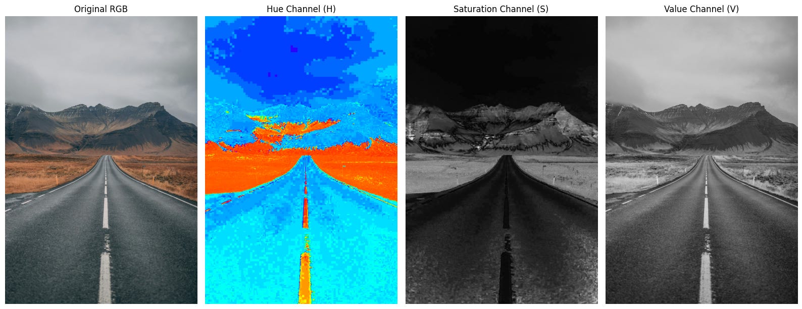
While RGB is the most common model for representing color in digital images, it is not always the most intuitive for image analysis. An alternative, widely used in computer vision and graphics, is the HSV color space—Hue, Saturation, and Value. This model separates chromatic content from intensity, offering a representation that aligns more closely with human perception.
In HSV, each pixel is described by three components:
Hue (H): Represents the dominant wavelength of the color—such as red, green, or blue.
Saturation (S): Measures the purity of the color, indicating how much white light is mixed in.
Value (V): Refers to the brightness or luminance of the color.
This separation allows for more perceptually meaningful adjustments. For example, changing the value affects brightness without altering the hue, and modifying saturation adjusts color intensity without impacting lightness. Such flexibility is particularly useful in image analysis tasks where lighting conditions vary, as HSV enables better isolation of color features from illumination effects.
Transforming an RGB image into HSV is a common preprocessing step in computer vision. Unlike RGB, which is perceptually nonlinear, HSV follows a more natural gradient of color change. This makes it easier to perform operations like segmentation, object tracking, and feature detection based on color, especially in environments where lighting is inconsistent or dynamic.
By decoupling color from intensity, HSV provides a more robust framework for interpreting and manipulating images in a way that mirrors how humans perceive visual scenes.
Greyscale Image Representation and Its Role in Analysis
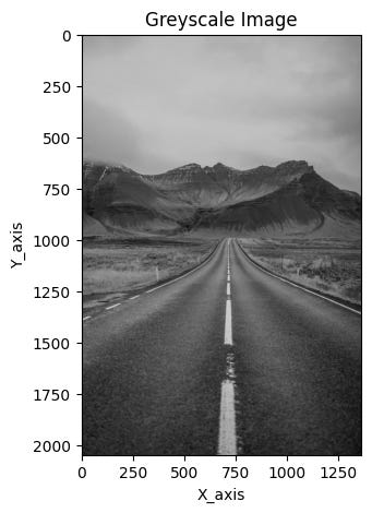
In its simplest form, a digital image can be represented by assigning a single numerical value to each pixel. This value reflects the signal intensity at that specific location, forming a 2D array of numbers. When visualized, these values are typically displayed using a color map—the most common being greyscale.
Greyscale, or intensity images, are composed of pixels that each carry one value representing brightness. Unlike color images, which use multiple channels to encode chromatic information, greyscale images reduce complexity by focusing solely on luminance. This simplification makes them highly efficient for many image analysis tasks.
Converting a color image to greyscale is often the first step in computer vision workflows. While this process reduces the amount of data, it preserves most of the critical features needed for analysis—such as edges, regions, blobs, and junctions. These structural elements are essential for understanding the geometry and layout of visual scenes.
As a result, many feature detection and processing algorithms operate on greyscale images. By stripping away color information, these algorithms can focus on shape, contrast, and spatial relationships, making the analysis faster and more robust. Greyscale representation thus serves as a powerful tool in simplifying visual data while retaining the essence of what makes an image informative.
From Analog to Digital: Sampling and Quantization in Image Creation
Creating a digital image begins with converting continuous data sensed by a device—such as a camera—into a format that computers can process. This transformation involves two key steps: sampling and quantization, both of which are essential to digitizing visual information.
Sampling refers to the process of digitizing the spatial coordinates of an image. It involves selecting specific points from the continuous signal to form a grid of pixels. The sampling factor, denoted as n, determines how frequently these points are taken—for example, sampling every 2 pixels along each line. This step defines the resolution of the image and how finely the visual scene is captured.
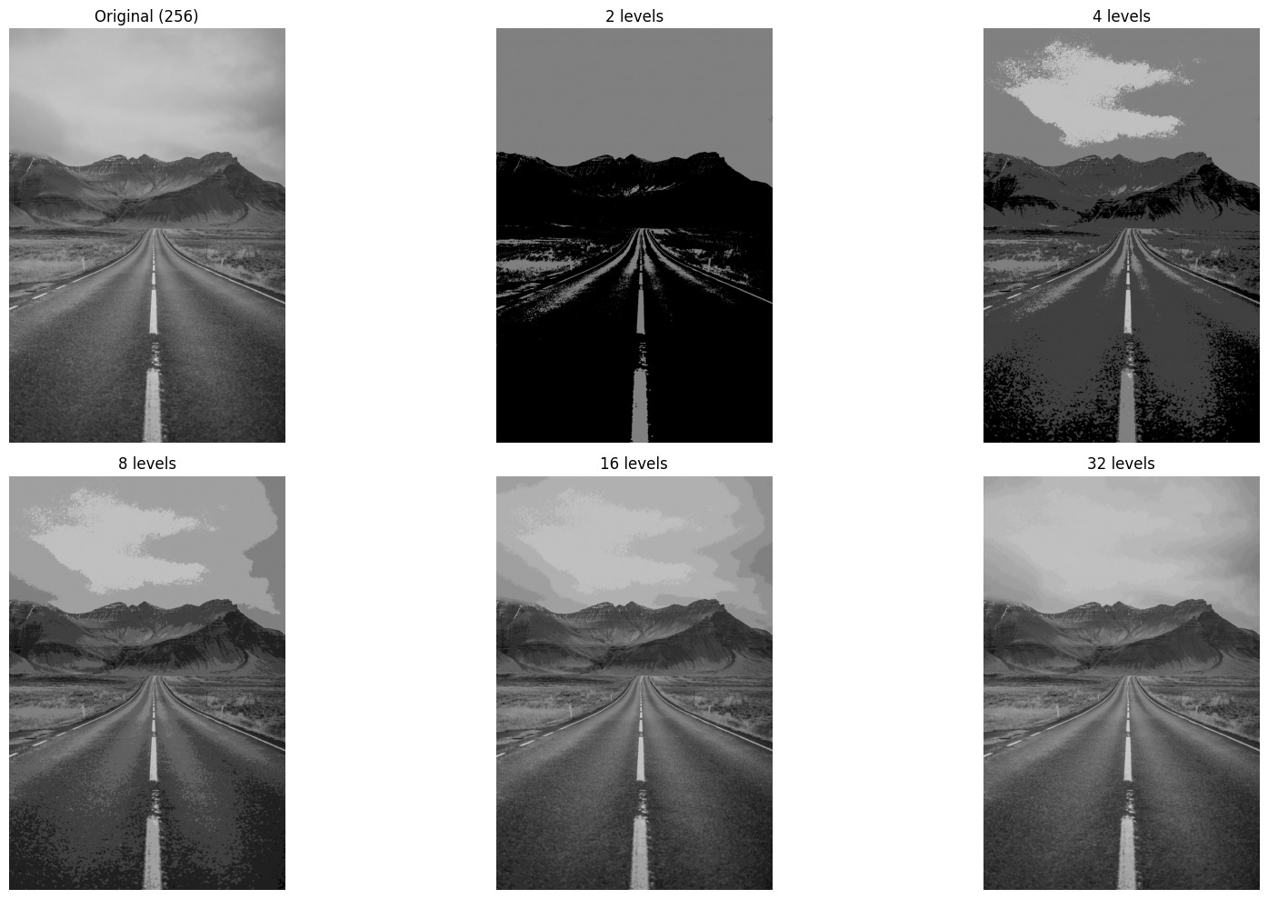
Quantization, on the other hand, deals with the amplitude values—such as brightness or color tones—at each sampled point. Using a quantization factor m, the continuous range of values is mapped to a finite set of discrete levels. For instance, a quantization factor of 2 would reduce the image to just two tones, such as black and white.
To illustrate, imagine sampling an image with a factor of 2 (every second pixel) and quantizing it with a factor of 2 (limiting it to black and white). The result is a simplified digital image that retains the basic structure of the original scene but with reduced detail and tonal variation. This simplification is often necessary for efficient storage, transmission, and processing—especially in applications where speed and resource constraints are critical.
Together, sampling and quantization form the backbone of digital image creation, enabling continuous real-world scenes to be represented in a format suitable for computer vision and image analysis.
Image sampling example:
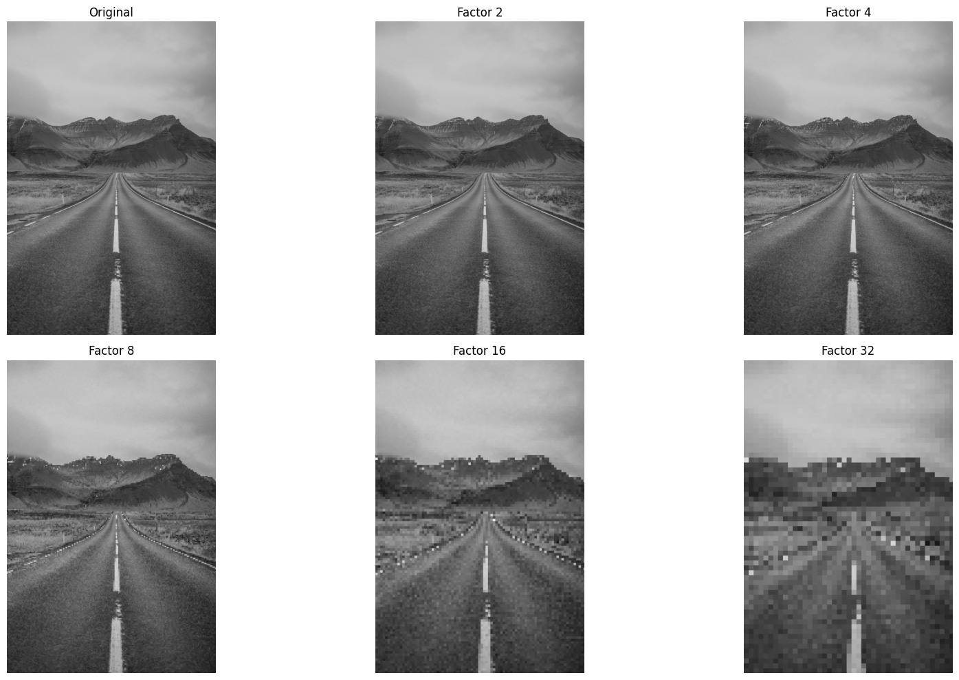
Image quantization example:
Bit-Plane Slicing: Revealing the Layers of an Image
Bit-plane slicing is a powerful technique in digital image processing that allows us to explore the visual significance of individual bits within each pixel. While it may seem abstract, this method provides valuable insights into how image data is structured and how different bits contribute to the overall appearance of an image.
Consider an 8-bit grayscale image, where each pixel can take on an integer value between 0 and 255. This value is stored as an 8-bit binary number, meaning each pixel contains eight bits of information. Bit-plane slicing involves separating these bits into eight distinct binary images, or “planes,” each representing a specific bit position across all pixels.
The first bit plane corresponds to the most significant bit (MSB), which has the greatest influence on the pixel’s intensity. Subsequent planes represent progressively less significant bits, down to the least significant bit (LSB), which contributes the smallest amount to the overall value. By displaying each bit plane individually, we can observe how much visual structure is retained at each level.
This technique is particularly useful for tasks like image compression, watermarking, and feature extraction. For example, higher-order bit planes often preserve the essential shapes and edges in an image, while lower-order planes may appear as noise. Bit-plane slicing thus offers a unique lens through which to analyze and manipulate image data at the binary level.
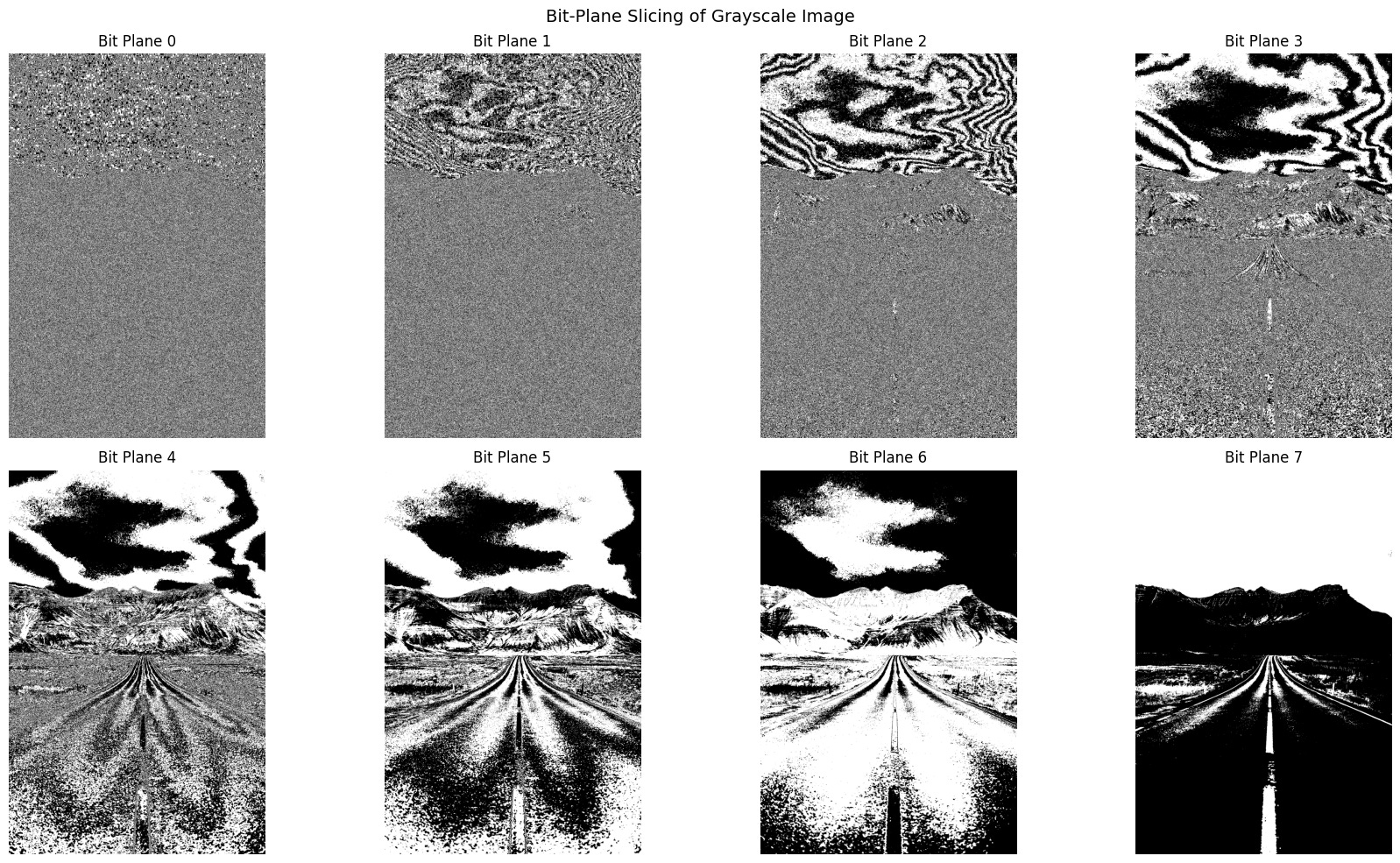
Image Compression: Balancing Efficiency and Fidelity
Bit-plane slicing offers a compelling insight into how certain image data can be removed without noticeably affecting visual quality. This principle underpins many image compression techniques, which aim to reduce file size while preserving the essential appearance of the image. If specific details are visually redundant—meaning they contribute little to human perception—they can be omitted from transmission or storage without compromising the viewer’s experience.
Redundant information typically falls into two categories. First, it may involve fine image detail, such as the least significant bits in pixel values, which often have minimal impact on overall appearance. Second, it may involve reducing the number of color or grey levels in a way that is imperceptible to the human eye. These strategies allow for significant data reduction while maintaining visual integrity.
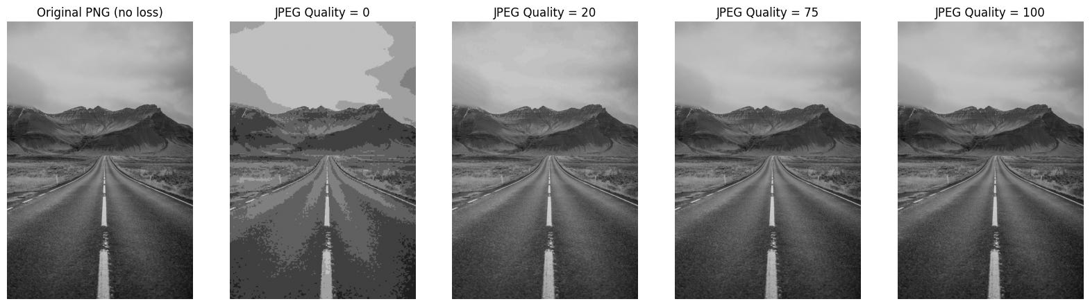
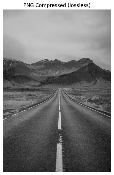
Image compression algorithms leverage these principles to store images more efficiently. There are two primary types of compression: lossless and lossy. Lossless compression retains all original data, enabling perfect reconstruction of the image. Formats like PNG and TIFF often use this method, making them ideal for applications where fidelity is critical.
Lossy compression, on the other hand, sacrifices some detail to achieve greater reductions in file size. JPEG is a common example, widely used for web and multimedia applications. While lossy methods may discard subtle variations in color or texture, they are designed to preserve the image’s overall appearance as closely as possible. The trade-off between storage efficiency and image quality is central to choosing the right compression strategy for a given task.
Conclusion
Digital image processing is a multifaceted discipline that bridges the gap between raw visual data and meaningful interpretation. From the foundational concepts of pixels and color models to advanced techniques like bit-plane slicing and perceptual color spaces, each layer of processing plays a vital role in how machines understand and manipulate images. Whether simplifying data through greyscale conversion or optimizing storage with compression algorithms, the goal remains the same: to extract, enhance, and utilize visual information in ways that are both efficient and perceptually relevant.
As computer vision continues to evolve, the interplay between low-level and high-level processing becomes increasingly important. Low-level methods prepare and refine the image, while high-level techniques aim to replicate human cognition—interpreting scenes, recognizing patterns, and making decisions. Together, these approaches form the backbone of modern visual computing, enabling applications that range from medical imaging and autonomous vehicles to digital art and augmented reality.
Understanding these principles not only deepens our appreciation of how machines “see” the world but also equips us to design smarter, more responsive systems that interact seamlessly with the visual environment.
M-a pus pe ganduri, cum anticipati ca va evolua discretizarea pentru aplicatiile viitoare, felicitari pentru articolul asta util.